Example 3: Loading from a file

This example demonstrates how to solve a Distance-based Critical Node Problem (DCNP) by loading an existing instance from a file. The DCNP adds a hop distance constraint to the standard CNP.

Problem description

The Distance-based Critical Node Problem (DCNP) extends CNP by considering hop distance. Two nodes are considered “connected” only if their shortest path distance is strictly less than a predefined hop distance limit b. This models scenarios where only nearby nodes can influence each other.

In this example, we:

Load a DCNP instance from an edge list format file
Set the budget to 10% of the total nodes
Use the BCLS (Betweenness Centrality Late Acceptance Search) strategy
Solve with a time-based stopping criterion

Loading the instance

PyCNP supports reading problem instances from files in two formats: adjacency list and edge list. The read() function automatically detects the format:

from math import floor
from pycnp import Model, read
from pycnp.MemeticSearch import MemeticSearchParams
from pycnp.stop import MaxRuntime
from pycnp.visualization import visualize_graph

# 1. Load an existing DCNP instance from a file
problem_data = read("Hi_tech.txt")
model = Model.from_data(problem_data)

Creating the model

We create a model from the loaded problem data:

# Create a model from the problem data
model = Model.from_data(problem_data)

Configuring problem parameters

For DCNP, we need to specify the hop distance limit. In this example, we set the budget to 10% of the total nodes:

# 2. Configure problem parameters
problem_type = "DCNP"
budget = floor(0.1 * problem_data.num_nodes())  # 10% of nodes
seed = 49
stopping_criterion = MaxRuntime(5)  # Stop after 5 seconds

Configuring the memetic algorithm

For DCNP problems, the BCLS (Betweenness Centrality Late Acceptance Search) strategy is recommended. We use fixed population sizing (no variable population) in this example:

# 3. Configure memetic search with problem reduction
memetic_params = MemeticSearchParams(
    search="BCLS",           # Betweenness Centrality Late Acceptance Search
    is_problem_reduction=True,  # Use RSC crossover
    is_pop_variable=False,   # Fixed population size
    initial_pop_size=5,
    reduce_params={"search": "BCLS", "beta": 0.9}
)

The reduce_params dictionary configures the RSC (Reduce-Solve-Combine) crossover:

search: Local search strategy used within RSC
beta: Fraction of common nodes to preserve (0.9 means 90% preservation)

Solving the problem

We solve the DCNP instance with a hop distance constraint:

# 4. Solve the instance via FTMS (Fixed Population Memetic Search)
result = model.solve(
    problem_type,
    budget,
    stopping_criterion,
    seed,
    memetic_params,
    hop_distance=3,  # DCNP: nodes within 3 hops are considered connected
    display=True,
)

The hop_distance parameter specifies the maximum hop distance for DCNP connectivity. Two nodes are considered connected only if their shortest path distance is less than this value.

Results

After solving, we can access the solution:

print(f"Removed nodes: {result.best_solution}")
print(f"Remaining connectivity: {result.best_obj_value}")
print(f"Number of iterations: {result.num_iterations}")
print(f"Runtime: {result.runtime:.2f} seconds")
print(f"Best solution found at: {result.best_found_at_time:.2f} seconds")

You obtain output similar to:

Removed nodes: {1, 18, 20}
Remaining connectivity: 293
Number of iterations: 92
Runtime: 5.02 seconds
Best solution found at: 0.18 seconds

Understanding the output

best_solution: Set of node IDs removed from the graph
best_obj_value: Pairwise connectivity considering hop distance constraints
num_iterations: Number of algorithm iterations performed
runtime: Total execution time in seconds
best_found_at_time: Time when the best solution was discovered

Visualizing the result

PyCNP provides an interactive graph visualization:

# 5. Visualize the result
visualize_graph(
    problem_data=problem_data,
    critical_nodes_set=result.best_solution,
)

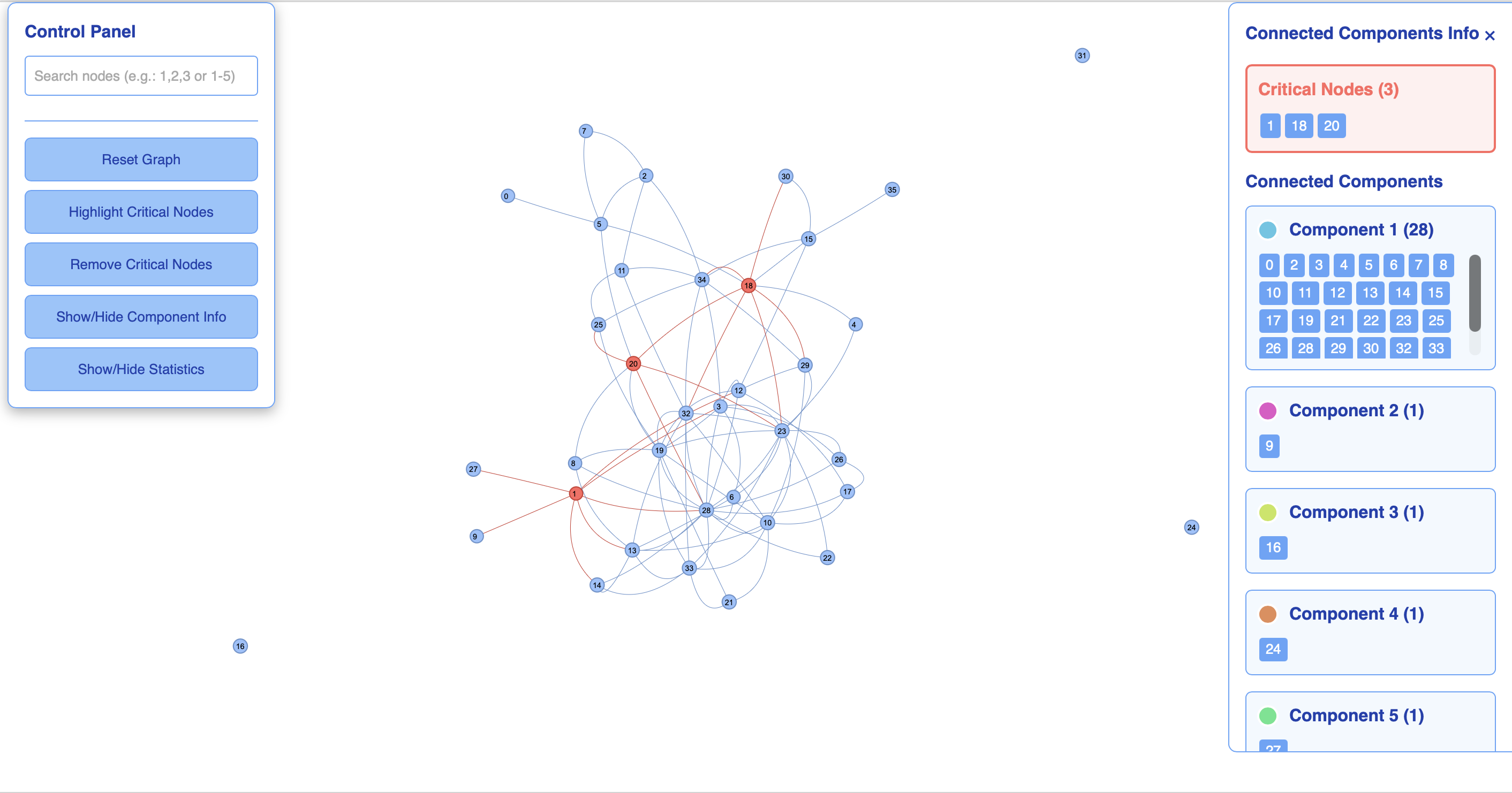
The visualization shows the original graph with critical nodes highlighted in a different color.